Content with notebooks

You can also create content with Jupyter Notebooks. This means that you can include code blocks and their outputs in your book.

Markdown + notebooks

As it is markdown, you can embed images, HTML, etc into your posts!

You can also \(add_{math}\) and

\[ math^{blocks} \]

or

\[\begin{split} \begin{aligned} \mbox{mean} la_{tex} \\ \\ math blocks \end{aligned} \end{split}\]

But make sure you $Escape $your $dollar signs $you want to keep!

MyST markdown

MyST markdown works in Jupyter Notebooks as well. For more information about MyST markdown, check out the MyST guide in Jupyter Book, or see the MyST markdown documentation.

Code blocks and outputs

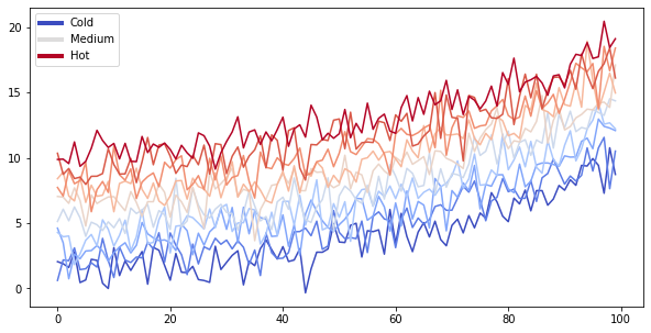
Jupyter Book will also embed your code blocks and output in your book. For example, here’s some sample Matplotlib code:

from matplotlib import rcParams, cycler
import matplotlib.pyplot as plt
import numpy as np
plt.ion()

<matplotlib.pyplot._IonContext at 0x10a5c94f0>

# Fixing random state for reproducibility
np.random.seed(19680801)

N = 10
data = [np.logspace(0, 1, 100) + np.random.randn(100) + ii for ii in range(N)]
data = np.array(data).T
cmap = plt.cm.coolwarm
rcParams['axes.prop_cycle'] = cycler(color=cmap(np.linspace(0, 1, N)))


from matplotlib.lines import Line2D
custom_lines = [Line2D([0], [0], color=cmap(0.), lw=4),
                Line2D([0], [0], color=cmap(.5), lw=4),
                Line2D([0], [0], color=cmap(1.), lw=4)]

fig, ax = plt.subplots(figsize=(10, 5))
lines = ax.plot(data)
ax.legend(custom_lines, ['Cold', 'Medium', 'Hot']);

There is a lot more that you can do with outputs (such as including interactive outputs) with your book. For more information about this, see the Jupyter Book documentation

import numpy as np
import matplotlib.pyplot as plt
%matplotlib inline

# Fixing random state for reproducibility
np.random.seed(19680801)

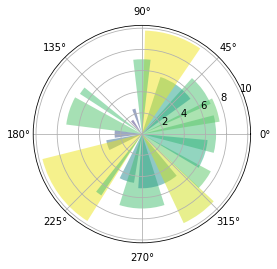
# Compute pie slices
N = 20
θ = np.linspace(0.0, 2 * np.pi, N, endpoint=False)
radii = 10 * np.random.rand(N)
width = np.pi / 4 * np.random.rand(N)
colors = plt.cm.viridis(radii / 10.)

ax = plt.subplot(111, projection='polar')
ax.bar(θ, radii, width=width, bottom=0.0, color=colors, alpha=0.5)

plt.show()

import numpy as np
import matplotlib.pyplot as plt

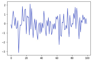
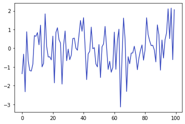
ϵ_values = np.random.randn(100)
plt.plot(ϵ_values)
plt.show()

ϵ_values = np.random.randn(100)
plt.plot(ϵ_values)
plt.show()

https://github.com/executablebooks/quantecon-mini-example https://executablebooks.github.io/quantecon-mini-example/docs/python_by_example.html

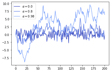
α_values = [0.0, 0.8, 0.98]
T = 200
x = np.empty(T+1)

for α in α_values:
    x[0] = 0
    for t in range(T):
        x[t+1] = α * x[t] + np.random.randn()
    plt.plot(x, label=f'$\\alpha = {α}$')

plt.legend()
plt.show()